 |
Exploration for oil and gas has been increasing dramatically in the deepwater, ultra-deepwater and shelf region of the Gulf of Mexico and other regions around the world (for example North Sea in Europe). A key technology component that helps to identify possible hydrocarbon targets as well as reduce the risks associated with such deep water exploration is seismic imaging. Seismic imaging helps to accurately position, define and delineate prospective complex subsurface structures before the dollar intensive drilling operations start. The average cost of drilling a well in the Gulf of Mexico is in the range of $50 million. Thus there is a huge emphasis on using seismic imaging to accurately define the shape of these complex subsurface structures and define the velocity variations in the surrounding regime before drilling operations commence.
Seismic imaging for oil and gas exploration is among the most computer-intensive commercial applications that exist for the scientific high-performance computing sector. The accurate reconstruction of 3-D images of the subsurface from 3-D seismic data requires the handling of huge data volumes, usually in the order of 10-15 terabytes, as well as application of computationally intensive imaging algorithms. Only large scale parallel computers can apply these algorithms effectively to image modern seismic data and deliver the results within a useful turn-around time. Thus using and harnessing cluster resources effectively is a crucial and integral component for the energy industry.
This chapter gives some examples along with the various issues related to the use of cluster computing for solving some of today's 3-D seismic imaging problems.
The first topic that is discussed addresses the I/O performance for seismic imaging application. For seismic imaging applications I/O issue as it turns out is a major bottleneck. Seismic datasets consisting of digitally recorded pressure waves can be very large (in the order of tens of terabytes). Thus it is not possible to read and store all the data and the required information in the memory at the same time. The data is therefore partially read and intermediate results are written out. This clearly indicates that I/O issues are extremely important in seismic imaging. The first case study that is described here discusses a strategy for improved I/O handling in a parallel architecture. The case study highlights the use of a parallel I/O system compared to the traditional standard I/O call and shows an improvement in performance of seismic imaging algorithms by almost an order of magnitude.
The processor and communication speeds of parallel computers have steadily increased. However the technology for increasing the I/O subsystems has not increased at the same rate. These are not well designed to efficiently handle massive I/O requirements like in seismic imaging. Most clusters generally use NFS file systems and MPI (message passing interface) as message passing libraries. The essential disadvantage of using NFS is that the I/O nodes are driven by standard UNIX read and write calls which are blocking requests. This is not a serious problem when the I/O volume is small, but when the volume increases as with seismic imaging applications it is important that the computations can be overlapped with I/O calls to maintain the efficiency. The main reason for poor application-level I/O performance is that most parallel I/O systems are unable to handle efficiently small requests, while parallel applications usually make many small I/O requests. Also another limitation of MPI-1 is that the I/O operation can be done only by the master processor, so while the huge amount of data is read by the master from the input file the workers remain idle. This also leads to an overhead of data distribution by the master to the workers.
This section will describe a strategy developed to handle such a specific I/O need in the seismic imaging industry known as ROMIO (high performance portable MPI-IO). It has been developed for a clustering environment where each machine has its own disk and processor so that each processor can do a local read and write. The process that is described here is a finite difference based 3-D post stack migration (imaging) algorithm with parallel I/O on a distributed memory parallel computer.
The imaging algorithm that will be used is a finite difference based depth migration algorithm for solving a parabolic partial differential equation in the frequency-space domain. This is a standard approximation for the scalar wave equation routinely used by the energy industry. The system is solved using a Crank Nicholson scheme with absorbing boundary conditions on the side. To solve the system the wavefield is decomposed into its monochromatic components by means of a temporal Fourier transform. The parabolic form of the scalar wave equation is then used to downward propagate each of the individual monochromatic waveform. An important advantage of this method is that it is naturally parallel in the frequency domain. Thus each frequency component can be individually extrapolated in depth, independently on each processor and there is no need of ant intertask communication. To set up the computation the input seismic data is first Fourier transformed w.r.t time and stored in a frequency sequential format. Only the required number of frequencies need to be stored, depending on the bandwidth requirement. This forms the input for the computational task along with the velocity model.
The standard parallel implementation is analogous to Master-Worker system. After reading all the required parameters, the Master determines the number of frequencies and frequency bandwidth to be assigned to each Worker. Then it reads and sends the frequency data to the designated Worker. Then the migration algorithm runs through the depth steps. The required velocity data for that depth step is sent to the Workers. Also the migrated data from all the Workers for that depth is collected by master, imaged and stored on the disk. The figure only shows one Master task and one Worker task, but in reality there are many Worker tasks. All the Worker tasks communicate with Master task in an identical fashion as shown in the figure.
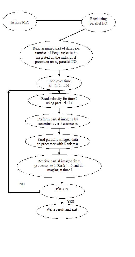
However the above standard method of implementing this algorithm is not robust in terms of the I/O handling. Instead of the standard way of dealing with the I/O issues for this problem this section outlines a method of dealing with the I/O issues using a parallel implementation. The parallel implementation is analogous to SPMD (Single Program Multiple Data) system. Processors read all the required parameters and read the frequency data that is to be migrated by the individual processor, in parallel. Then the migration algorithm runs through the depth steps. All processors read the required velocity data for that depth step in parallel. The processor with rank zero, collects the migrated data from all the processors for that depth, images it and the stores it on the disk. A flow chart of this algorithm is shown in figure 1.
Even though the developed codes for ?-x depth migration (with and without parallel I/O) are portable across various platforms, most of the development was done on PARAM 10000. The PARAM 10000 system has 40 SUN E450 compute nodes, each with 4 processors @300MHz. Out of 40 nodes 4 nodes are network file servers with 1GB RAM and 512K cache. High-speed network such as fast Ethernet with peak bandwidth 100MB/s connects the nodes. Following tables show the comparison between execution time for ?-x depth migration algorithms with and without parallel I/O for various small and large sized data sets.
2-D Depth Imaging
Size of FFT Data: 2.66 Mb
Size of velocity model: 1.824 Mb
Total number of frequencies used: 222
Execution time with 16 processors
Without parallel I/O: 57.8 seconds
With parallel I/O: 37.6 seconds
3-D Depth Imaging, Dataset 1
Size of FFT Data: 60 Mb
Size of velocity model: 75 Mb
Total number of frequencies used: 420
Execution time with 24 processors
Without parallel I/O: 5765 seconds
With parallel I/O: 4331 seconds
Execution time with 64 processors
Without parallel I/O: 2301 seconds
With parallel I/O: 1645 seconds
3-D Depth Imaging, Dataset 2
Size of FFT Data: 1.3 Gb
Size of velocity model: 1.2 Gb
Total number of frequencies used: 256
Execution time with 64 processors
Without parallel I/O: 43500 seconds
With parallel I/O: 28370 seconds
The execution time charts given above show that with parallel I/O implementation the seismic imaging algorithm takes almost 30% less time compared to the standard I/O implementation. The reason for this improvement is the change in communication that is possible with the support of parallel I/O. In the case of parallel I/O, the communication involved in the reading and distributing the data among processors can be changed to just reading the data in parallel by the processors without any communication involved. The communication comes at the end of the algorithm, when the final imaging takes place.
In the seismic industry, where the amount of data that needs to be processed is often measured by the number of tapes, which amount to hundreds of gigabytes and now terabytes, the improvement of making efficient use of the I/O subsystem becomes increasingly apparent. A 10% to 20% improvement in runtime would amount to saving of millions of dollars in processing time. The case study discussed above highlights a step in this direction.
1. Claerbout. J., Imaging the Earth's Interior, 1985, Blackwell Publications
2. S. Phadke, D. Bharadwaj and S. Yemeni, Wave equation based migration and modeling algorithms on parallel computers., Proc. of SPG , 1998.
This case study shows how seismic modeling can benefit from PVM (Parallel Virtual Machine) techniques by describing a message passing implementation of DSO, the modeling and inversion code developed in The Rice Inversion Project using PVM3, that runs on a network of workstations. The study uses coarse grain parallelism, of SPMD type in which the individual tasks are full edged simulations. Thus, even though the amount of data needed by each task is substantial, the length of the computation is such that it is reasonably possible to offset the time taken by the communications.
DSO (Differential Semblance Optimization) is a code for seismic inversion under development in the Rice Inversion Project, which can be viewed as doing simulation, or data-fitting, of multi-experiments. DSO tries to find a model that best explains observed data, by using a variant of the least-squares technique. It assumes that these data are produced by one physical model, but come from a suite of experiments done by varying some additional parameter. The basic DSO idea is to let part of the model depend on this parameter, but to penalize the objective function in so that the optimal solution will actually be independent of the parameter. This study illustrates two different examples, the first one from is an acoustics point-source experiment, the second one, written at Exxonmobil describes viscoelastic plane-wave propagation.
In the first example, the earth is described by its velocity (assumed smooth), and its reflectivity (assumed rapidly varying), and the additional parameter is the position of the seismic source. DSO lets the reflectivity depend on shot position, but since there is only one earth,it penalizes to ensure the solution does not actually depend on it. This is in some sense a canonical example, and most of the terminology derives from it. Thus the additional parameter is invariably called a shot.
For the second example, the earth is now visco-elastic but one-dimensional, the source is a plane wave and the additional parameter is the angle of incidence of the plane wave. Again, some of the quantities are artificially allowed to depend on the angle of incidence, and this dependence is penalized. As a consequence of this discussion, we see that the main computational task of DSO is the simulation of a large number of instances of a basic experiment, under different conditions. All these simulations are independent, and it is quite natural to process them simultaneously.
For the first example above, a simulation is the solution of the wave equation with several right hand sides, each one corresponding to a different seismic source position. For the second example, simulation is done for the arrival of plane waves with different angles of incidence. The implementation of DSO is built around the principle that generic tasks should be coded in a generic way. A consequence is that the simulator is completely hidden from the optimization algorithm. This allows the use of the same inversion method with several different choices of propagation models. This allows code at a very high level: a simplified view reduces to two routines, destined to be cooperating processes:
Since all instances of shot are independent, it is a very natural idea to run them in parallel. Such an approach to parallelism has several potential advantages which are:
A manager - worker implementation suggests itself, with simline acting as the manager, or rather as a work dispatcher, and each incarnation of shot as a worker, simply treating shot after shot.
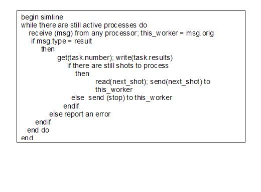
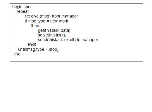
This implementation has the additional advantage of providing free load-balancing. A fast worker will require (and receive) more work than a slower one, without the manager having to be concerned about balancing work between workers. One drawback is the possible bottleneck of having the manager do all of the I/O. But as we shall see on examples (section 4.2), this does not usually happen, and we even get overlap of the communication by the computation. We show below the pseudo-code for both the manager and the worker sides. We denote the number of tasks by ntasks, and the number of processors by nprocs. The algorithm for simline (the manager) is shown on figure 1. The main loop of simline is very simple: it waits for a message to arrive. In normal operations, this should be a worker reporting work done. The results are then stored, and if there are more tasks to process, simline reads the relevant data, and sends them the worker. Otherwise, simline simply sends a stop" signal. A feature that is not shown in figure 1 is that there is also simple for of read-ahead that is implemented, before entering its main loop, the manager starts by sending two tasks to each worker, thus ensuring that when a worker requests a new task, one is already there waiting. Obviously, the success of this scheme hinges on the assumption that it takes longer to compute a task than to send it. Figure 2 shows the pseudo-code for shot. Its structure is even simpler. After having received initial information, it waits for work to arrive from simline, performs the corresponding computation, and goes back to wait for the next message. Hopefully, the prefetching outlined before is efficient, so that shot is never blocked on the receive statement.
The previous section showed the basic algorithm used. For a practical implementation, it is important to choose a proper transport mechanism, in other words to specify how different processors communicate. Use of Remote Procedure Calls, and the UNIX mail system are not adequate because of the large amount of data to be exchanged. Instaed this study uses PVM as our message passing mechanism, because of its wide availability, and also because it is rapidly becoming a de facto standard for distributed applications. Its allows a heterogeneous network of computers to appear as one single distributed memory computer. PVM is composed of a daemon than enables PVM to run on a given machine, and of a user-callable library of routines that allow the user to start tasks on remote machines, send and receive messages between different processors, and provides tools to manage these different processes.
Two important features of PVM of which this study made particular use are:
Assessing the performance of any program is difficult, and programmers are notoriously poor at guessing where to optimize a code. This is even more true of parallel programs, where it is compounded by the necessity to take into account not only the computations but also the communication delays. Tools are essential in order to achieve an understanding of the kind of performance we are getting out of a code, and of the bottlenecks.
An essential aspect of parallel programs is their dynamic character. Accordingly, a visual display of the time evolution of the program is important. This requires the code to be instrumented, then log-files are created while the program runs (hopefully with a minimum impact on the behavior of the program), and the log-files are interpreted graphically a-posteriori. The tools used here are two packages working together: alog is used to instrument the code. It allows the user to define events, to be logged to a _le. The second package, upshot, interprets the log-files in a graphical way using the X Window System.
The first example is an adjoint map on a scaled-down version of the so-called Marmousi" model. We used 24 shots, on a 1650_450 grid, with 1450 time steps. This experiment was performed at the IBM Center in Dallas, on a cluster of 8 RS600 370 workstations, of which one acted as the manager (no worker ran on the manager node). The time and Mops rate on a single node were 624 s and 40 Mops. The time with 6 workers is 45 mins 24 s, giving a speedup of 4.4 (or an efficiency of 72 %).
The geophysical implications of this example consists of a low velocity perturbation in an otherwise layered medium. The experiment consists of simulating 30 shot positions, on a 512 by 128 grid. There are 500 time steps, and 34 receiver positions. This is representative of the model sizes we are currently able to use for inversion, as shown in the next subsection. We first ran on a single node to evaluate floating performance of the chip. The execution time was 527 s, the elapsed time was 560 s, or 94% use of the machine. On a Cray Y-MP (at Cray Research Corporate Computing Network), execution time was 83 s. The Mops rate were 254 on the Y-MP, and 40 Mops on the RS6000.
Then, the cluster was used, using 6 workers in addition to the manager. Execution time was 130 s. Both alog and upshot were used to produce and examine a log files for this run. The log files show that the workers are busy computing most of the time. Also, the master has only bursts of activity, when it is doing I/O. This is the expected behavior, and justifies the design decisions, at least for doing simulations.
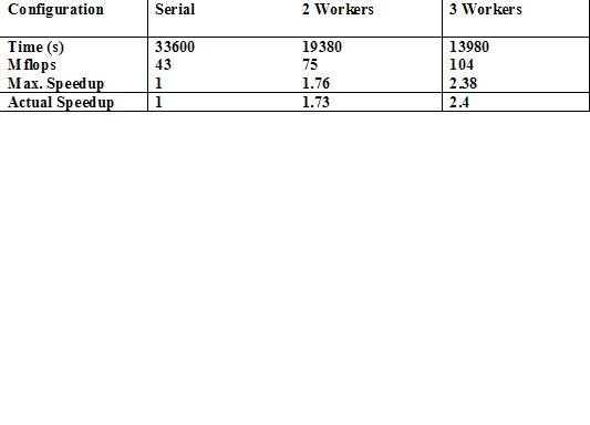
For this example, the physical model is the same as in 3.2, but now inversion will be attempted. This includes a significant amount of linear algebra which is not parallelized. Note that a run in this section is the equivalent of 58 runs of the previous section. This task was ran on a dedicated cluster of 4 IBM RS600 workstations, connected by a 10 Mb/s Ethernet. Performance results are shown in the table below (maximum speedup is computed from Amdahl's law and actual speedup is what was actually measured).
An important point to remember is that Amdahl's law has not been violated, instead this scheme has benefited from super-linear speedup due to computation and I/O overlap, which is not taken into account by Amdahl's law. In this case, again, the workers were kept busy all the time, their loads were balanced, and communication costs were insignificant
The above case study presents a task level parallel implementation of DSO. The study described the implementation, given the rationale on which it is built, and also presented some preliminary evidence that the design works, at least for modeling. The method however has limitations for doing inversion.
1. W.W. Symes and J.J. Carazzone, Velocity inversion by differential semblance optimization, Geophysics, volume 56, 1991.
This case study demonstrates how performance of complex algorithms can be improved by redesigning the code structure of such algorithms. The study uses an example of a seismic imaging algorithm to demonstrate techniques that can be used to attain improved performance on existing hardware including parallel and distributed systems.
Along with development of sophisticated algorithms for a wide variety of tasks, there is also the need for developing methods that can effective use the avaialble machines and use thier full potential. This practise of best use of the hardware has been termed as performance programming.Performance programming is markedly different from the usual variety of coding. The primary goal of performance programmimg is to bridge the gap between the speed at which a code is running and the speed at which it should run when best optimized. This paper uses an example of a seimic imaging algorithm to demonstrate the efficiency that can be attined via performamce programming.
The basic function of a seismic imaging/migration algorithm is that it converts signals recorded on the surface to an image of the subsurface by extrapolating the wavefield recorded on the surface down into depth. there is a Fast Forier Trnasform (FFT) involved of the wavefield so that each frequency component can be extrapolated independently. The primary cost of this kind of an algorithm is the extraoplation step. In this study the extrapolation is done using a 39 point symmetric filter which makes the scheme very accuarate but computationally intensive. This is because to evaluate each sample of the wavefield at a particular location 39 samples from the previous location has to be used in a convolution like scheme. The following sections will describe how this algorithm can be bullet=proofed and enhanced using principles of performance programming.
One of the important component of this algorithm is an intensive inner loop where operations like using the filter for convolution is done. Unless this inner loop performance is optimized, efficiency cannot be achieved. This means that the code must make optimal use of the machine's underlying instruction set. The machine that has beed used for this study isa 20 MHZ IBM RISC system/6000 computer. This machine can perform 2 floating point operations per cycle so that is maximum theoretical speed is 40 Mflops. This seismic imaging method being implemented here has an inner loop that needs to do 6 floating point adds and 4 multiplies requiring 6 cycles. The maximum performance achievable is therefore 33 Mflops. There however exists a strange condition in the 6000 C compiler which treats a filter operation of the form x+ = a*b + c*d as x = x + (a*b+ c*d)i. Thus instead of having 6 operations we have eight. Thus a simple rearrangement of the C code will speed up performance by a factor of 10%. Another problem is that although the 6000 can dispatch a floating point instruction every cycle, the results are not available for atleast 2 cycles. This is also an area where drastic improvements can be achieved by simple restructing of the code. However this study could not achieve the optimal goal of 6 cycles per iteration. But with knowledge of the underlying machine hardware fine tuning resulted in achieving 7 cycles per iteration for the inner loop.
Another point of concern for the inner loop is the fixed ppoint computations. This can be optimized by structuring the code such that the computation does not require more than one address computation per floating point instruction. An example of this for the seismic migration code is the computation of imaginary numbers. It is necessary that the real and the imaginary parts are computed together in one loop rather that in separate loops as this halves the total number of loads and reduced redundant communications.
Along with the inner loop, the outer loop of seismic migration needs to be optimized as well. In the seismic migration algorithm, the outer loop involves substantial setup before the inner loop is reached. The setup involves data accessing, which may lead to cache miss. It also involves two float to fixed conversions which involves a 5 cycle delay. These problems can also be optimized by computing setup values one iteration in advance. This means that during iteration number j of the inner loop setup the iteration number (j+1) before beginning thr execution of tje inner loop. This permits muti-cycle delay transfers between units to be overlapped with useful work. This technique also leads to a 10% improvement in performance of the seismic imaging code.
Controls should also be made on the way data is moved between different levels of the memory hierarchy and also between processors.It is extremely important that cache and page misses are avoided. For example multi dimensional arrays should be accessed in a manner which reuses elements of the cache line before the line is moved out of cache. As fas as techniques for reducing communication overheads in the memory hierarchy is concerned, an useful strategy is to breakup the computation cube into subcubes that fit the hierarchy at various levels. Management strategy is improved significantly by processing subcubes that have small surface to volume ratio. Similar considerations must be applied when distributing a computation to multiple processors. Once the data management was properly introduced along with the implementation of the proper code structure the computation speed increased from 8 to 26 Mflops for the sequential computation.
The distributed system for this case study was a set of 6000 machines connecetd using token rings. The parallel impementation is done using a manager-worker organization, similar to a master-slave arrangement except that the workers request assignments as well. The workers repeatedly request assignments from the manager and process the work. Finally when there is no additional work to perform, the worker reports the result of their computations to the manager. This partail results are then accumulated by the manager and it then writes the output.
The computations are assigned to the workers by chopping or cutting the computation cube in the most efficient manner. For this case study it was found that chopping the cube perpendicular to the frequency axis is the most efficient way. For this chopping process to be fully efficient it is however necessary that each worker keeps a separate copy of x by z array (the other two dimensions of the cube). The parallelism is furter improved by recognizing that ideas from the previous section (particularly on how the inner loop was optimized) should be incorporated here. In this case the inner loop can be thought of as a sequential computation of the subcubes. While the setup procedure in this case deals with communicating the surfaces of these subcubes. Once this analogy with the sequential code is recognized all the techniques that were developed and used in the previous section can be now used here.
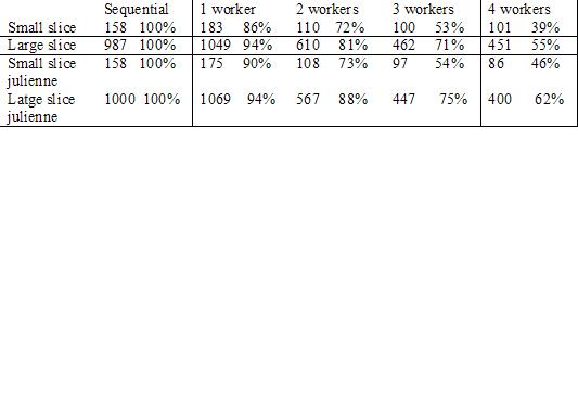
For the first det of results the subcubes or the work assignments are slices of the cube one frequency wide. The evaluation of this subcube requires the extrapolation table of seimic imaging, the velocity model (nx by nz matrix) and a row of frequency data (nx complex numbers).The first two rows of figure (1) shows the results obtained with a small (nx=467, nz=200,mw=228) dataset and a large (nx=1000, nz=400, nw=303) dataset. The table includes entries for runtime and utilization. Runtime is wall clock time on unloaded machines, while utilization is sequential runtime divided by the product of the number of workers and the runtime, expressed as percentage. The small-slice-at-a-time utilization figures are disappointing as distributing the computation seems to entail significant communication overhead. This overload was due to low effective bandwidth and this strategy failed to overlap this overhead with useful computation.
To overcome this problem a julienne strategy was then adapted, whose primary goal is to overlap communication with useful computation. For this the initial assignment to each worker should have a small surface area to allow rapid startip of all workers as well as a large volume so that the worker does not have a long wait before the manager is ready for the workers' next request. The surface to volume ratio of this initial assignment is minimized by sending twice as many velocity rows as frequency rows as the frequencies are complex. In this strategy the initial work assignment involved 25 frequency rows and 50 velocity rows. The manager sends 50 row swaths of the velocity matrix with each assignment until each processor has the entire velocity matrix. Thereafter the manager sends 25 row swaths of the frequency matrix. The results are shown in the third and fourth row. It shows a marked improvement in performance.
The julienne techniques can be further improved by using for example variable sized julienne strips. In this case study, the processor is idle when the worker is communicating with the manager. Thus placing two workers on the processor may allow further overlap. These strategies however have not been implemented in this study.
This Case study demonstrates that the performance of the seismic imaging code can be improved by a factor of 2 to 4 by exploiting knowledge of the architecture of the environment. This techniques of improving the performance apply at all levels of the machines, from the ALUs and registers to the memory hierarchy. Another important conclusion of this case study is that it is helpful to visualize a scientific computation as a multidimensional soild where the surface area corresponds to communication and the volume to computation.
1. G. Almasi, Parallel distributed seismic migration. In Proc. ACM Workshop on Parallel and Distributed computing, 1991
2.G.F. Grohoski. Machine organization of the IBM RISC System/6000 processor. IBM J. Res. Des., volume 34(1).
3.D. Hale, Stable explicit depth extrapolation of seismic wavefields, 60th Annual meeting, SEG, 1994.
4. H.S.Warren, Instruction scheduling for the IBM RISC System/6000 processor. IBM J. Res. Dev , volume 34, 1990.
We would very much appreciate comments, corrections or suggestions for additions:
linclusters (at) gmail.com
Copyright © 2005, LinuxClusters.com. All Rights Reserved.